F= C + 2 - P
and with F=2 & C=3, P = 3, which tells us that for this divariant assemblage, we will have three coexisting phases.
Mineral phases that coexist with each other at this temperature and pressure are connected by lines, called tie lines.
| EENS 2120 |
Petrology |
| Prof. Stephen A. Nelson |
Tulane University |
|
Triangular Plots in Metamorphic Petrology |
|
| Like igneous rocks, most metamorphic rocks are composed of 9 or more major
elements. Thus, initially it would appear that we are dealing with a
9 or 10 component system. Recall, however, that the number of
components in any given system is the minimum number required to define
the composition of all phases in the system. Thus, since
constituents like Na2O and K2O are not usually found
as separate mineral phases, we can combine these with other constituents,
like Al2O3 and SiO2 in the feldspars, and
thus reduce the number of components required to define our system.
This is especially important if we wish to graphically display chemical rock and mineral data in a way that is easily visualized. In fact, the best way to visualize such data is to attempt to reduce the number of components to 3, so that we can plot the compositions of rocks and minerals on a triangular composition diagram. Before discussing how this is done, we first review some of the principles of three component compositional diagrams. |
|
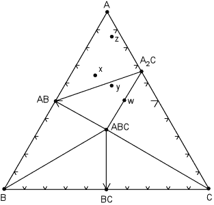
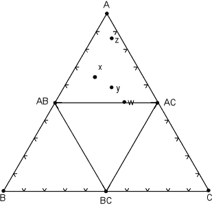
General Three Component Compositional Diagrams For the moment we will assume that we are in a true 3 component system and the minerals that we display on a triangular composition diagram is a set of mineral that are in equilibrium over a narrow range of temperature and pressure. We first look at how one of these diagrams might appear in the hypothetical system A, B, C. |
As shown on the diagram, at the pressure and temperature
under consideration, there are seven possible minerals that can occur in
this system, although we know from the phase rule that not all 7 can occur
in the same rock. In general, the most common set of phases will be
where the number of degrees of freedom, F, is 2, i.e. where pressure and
temperature can vary by small amounts without changing the number of
phases. For such a situation, the phase rule is:
and with F=2 & C=3, P = 3, which tells us that for this divariant assemblage, we will have three coexisting phases. Mineral phases that coexist with each other at this temperature and pressure are connected by lines, called tie lines. |
|
| The tie lines divide the diagram into smaller compositional triangles,
that tell us what minerals will coexist in a rock of any composition under
the current temperature and pressure conditions. For example, for a rock
with composition x , the divariant mineral assemblage is AB, A, A2C.
If the rock composition is moved slightly so that it now has composition
y, note that the mineral assemblage will change to AB, A2C,
ABC.
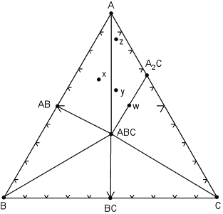
Within each compositional triangle, we can use the lever rule to estimate the proportions of the phases that will occur in the rock. For example, a rock with composition x will have the same mineral assemblage as a rock with composition z, but rock z will have a much higher proportion of the mineral A. In a rare case, note that it is possible for a rock composition to lie exactly on a tie line, for example the rock with composition w. Such a rock would consist of approximately equal proportions of the minerals ABC and A2C. Note that if we apply the phase rule to this situation, C=3 and P = 2, we find F = 3. But - in reality, because the number of components is defined as the minimum number required to form all minerals, we can see that rock w really lies in a 2 component system, rather than a 3 component system. So, F is still equal to 2. Similarly if a rock had exactly the same composition as mineral ABC, then it would only have 1 phase, ABC, present at this temperature and pressure and would be considered a 1 component system. We next illustrate what might happen to the mineral assemblages if we change the pressure and temperature condition to such that some of the mineral assemblages change. The same compositional triangle is shown in the diagram below, but note the shift in the tie lines. Instead of minerals AB and A2C coexisting, at the new conditions minerals ABC and A coexist. This forms new compositional triangles. |
| We can deduce form this that a chemical reaction must have occurred,
causing AB + A2C to react and be replaced by the minerals A +
ABC.
The chemical reaction breaks the tie line to form a new one, and the reaction can be written as:
Note that after the reaction has occurred, new mineral assemblages develop in the rock. Rock x is now composed of AB, ABC and A, rock y is now composed of A, A2C, and ABC, and rock z (which had the same assemblage as x in the previous diagram) now has the same assemblage as rock y, although, again, the proportions of the three minerals will be different in rocks y and z.. |
 |
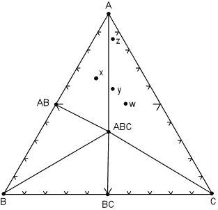
| The next case we consider is if one of the minerals reacts away completely because it is no longer stable under the new pressure and temperature conditions. This case is illustrated in the diagram below, where we note that the mineral A2C has reacted away. |
The reaction that has occurred is:
Note that now rock w, along with rocks y and z are in the three phase triangle A, ABC, C and will contain the minerals A, ABC, and C, although the minerals will occur in different proportions. Furthermore, rock x still has the same mineral assemblage - AB, ABC, A, as it had in the previous diagram. |
 |
| Another possible case is where a phase disappears and new phase appears as temperature and pressure change to new values. In the diagram below, a new phase, AC appears and mineral ABC disappears. |
At some point moving from the pressure and temperature conditions of the
diagram above to those of this diagram, the following reaction has taken
place:
Note that now, rocks x, y, and z all lie within the same composition triangle and have the same mineral assemblage - AB, AC, and A, although again, each rock has different proportions of these minerals. Rock w, is now in the 2 component system AB - AC. |
 |
| As we stressed in mineralogy and in our discussion of igneous rocks. Many minerals that occur in nature are solid solutions, and thus they can have a variable composition. Solid solution minerals, because of their possible range in chemical composition, do not plot at single point on the composition diagrams, but instead plot along a line or within a field that represents the possible range in chemical compositions. |
| When solid solutions are present, the tie lines become spread out over a
range of compositions as is seen in the diagram shown here for the
hypothetical system X, Y, Z.
In this diagram the mineral X(Y,Z) shows limited solid solution with variable amounts of Z substituting for Y. This is shown by a solid line extending from pure XY into the ternary diagram. Similarly, mineral X2(Z,Y) shows limited solid solution of Y substituting for Z. The minerals XYZss and Zss show a range of possible compositions that are represented by a shaded field on the diagram. |
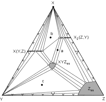 |
| The tie lines that connect the ranges for the solid solution
compositions are just some of an infinite array of possible tie
lines. But, note that a rock with a composition shown as "a" in the
diagram, will consist of two phases an X2(Z,Y) solid solution
and an XYZ solid solution. The compositions of these coexisting solid
solutions are indicated by the shaded circle at the end of the tie line
that runs through point a.
For rocks with compositions that plot in the 3 phase triangles, like b and c in the diagram, the mineral assemblage would consist of the three phases at the corner of the triangles. If solid solution minerals occur at one or more of the apices of the compositional triangle, then the composition of the solid solution mineral will be that found at the apex of the triangle. These solid solution compositions are shown as white filled circles. For example, a rock with composition c at the pressure and temperature of the diagram will be made up of Y, Zss, and XYZss. A rock with composition b will be made up of X(Y,Z), X2(Z,Y), and X. Common Triangular Plots Used in Metamorphic Rocks As stated above, common metamorphic rocks contain many more than the 3 components we would like to have for easy graphical description of composition and mineral assemblage. The 13 major elements (expressed as oxides) in most (not all) metamorphic rocks are SiO2, Al2O3, TiO2, FeO, Fe2O3, MnO, CaO, MgO, K2O, Na2O, P2O5, H2O, and CO2. Obviously if a rock consists only of one or two of these constituents, the problem is easy. For example, a pure Quartz sandstone would contain only SiO2, or a pure calcite limestone would contain only CaO and CO2. But, the more common rocks like shales, basalts, siliceous dolomites, or granites, are not so simple. There are various methods available to reduce the number of components to a workable number. Among these are: |
|
| ACF Diagrams
One of the first uses of these types of diagrams was by Eskola (1915) who employed a diagram known as the ACF diagram in his study of metamorphic rocks. To plot a rock on the ACF diagram, the chemical analysis of the rock is first recalculated to molecular proportions by dividing the molecular weight of each oxide constituent by the molecular weight of that oxide. Nominally, the ACF diagram plots the following components:
However, the A value we want is the value of excess Al2O3 left after allotting Na2O and K2O to form alkali feldspar. The CaO value we want is the excess CaO after allotting P2O5 to form apatite, assuming that any P2O5 in the rock will suck up CaO to form apatite. We will assume then that all mineral assemblages plotted may also contain alkali feldspar and quartz (and apatite). |
|
So, to obtain the plotting parameters, we calculate the following, where the bracket symbols [ ] indicate the molecular proportions of the oxides.
Since we are only plotting these 3 components, they have to be normalized so that they add up to 1 (or 100 if we are plotting %).
|
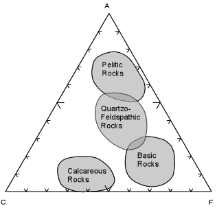
| When these calculations are done for a wide variety of rock
compositions and grouped as pelitic, quartzo-feldspathic, basic, and
calcareous, the fields are as shown here.
Most shales will plot in the field of Pelitic Rocks. Quartzo-feldspathic rocks like feldspathic sandstones, granites, and rhyolites will plot in the Quartzo-Feldspathic field. Basic igneous rocks, like basalts and gabbros will plot in the field of Basic Rocks, and siliceous limestones and dolomites will plot in the field of Calcareous Rocks. This diagram and the fields shown will become an important part of later discussions, so it is wise to know approximately where the fields of these different chemical types occur on the ACF diagram. |
 |
Plotting minerals on the ACF diagram is somewhat easier if you know the
chemical formula of the mineral, since mineral formulae are already
in the form of molecular proportions. Thus for a mineral like hypersthene,
(Mg,Fe)SiO3 , we have 1 molecule of (FeO + MgO) for every 1
molecule of SiO2. Thus:
and we see that hypersthene would plot at the F corner of the ACF diagram. As a second example, look at the formula for tremolite - Ca2(Mg,Fe)5Si8O22(OH)2 We can rewrite this formula as 2CaO 5(Mg,Fe)O 8SiO2 H2O then:
Other minerals are more complicated. For example, the formula for chlorite is (Mg,Al,Fe)12(Si,Al)8O20(OH)16. Thus we have several possibilities for writing the formula for chlorite, and depending on which formula we use, chlorite will plot at different locations on the diagrams. You will explore the possible solid solution ranges in a lab on this topic. |
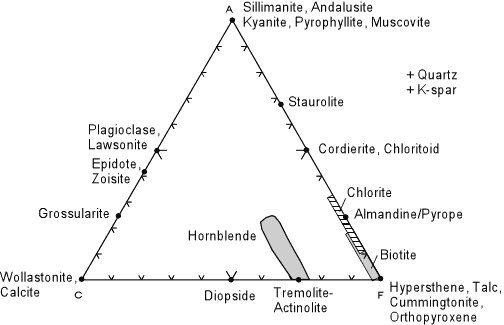 |
| Although you will calculate the plotting positions of some rocks and a wide variety of minerals in lab, the diagram above shows the plotting positions of some of the more common minerals that occur in metamorphic rocks. Note that this diagram is for reference only, it does not show mineral assemblages in rocks (there are no tie lines). Note that alkali feldspars do not plot in this diagram, but are assumed to be present because of the way we calculate the A component. |
| AKF Diagrams
In AKF diagrams we assume that both alkali feldspar and plagioclase feldspar can be present, thus the amount of Al2O3 that we use is the excess Al2O3 left after allotting it to all of the feldspars. To obtain the plotting parameters for ACF diagrams, calculate the following:
|
| Minerals are plotted in the same way as was done for the ACF diagrams, and an example AKF diagram showing the potting positions of common metamorphic minerals is shown below. |
 |
Note that K-feldspar plots in the lower right hand corner. To see why,
we first take the chemical formula of K-feldspar KAlSi3O8
and rewrite it in oxide form as 1/2K2O 1/2Al2O3
3SiO2. Then:
Another example is muscovite KAl3Si3O10(OH)2 or 1/2K2O 3/2Al2O3 3SiO2 H2O. For muscovite:
|
|
So,
|
| Note that AKF diagrams are used for CaO-poor, K2O-rich rocks,
whereas ACF diagrams should be used for Al2O3
and CaO - rich rocks.
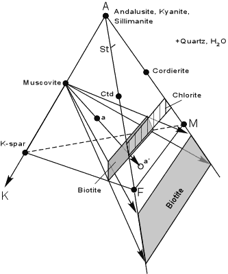
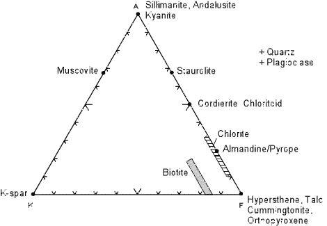
AKFM Projection onto AFM The ACF and AKF diagrams discussed so far, are fairly simple, but useful. One of the problems associated with ACF and AKF diagrams is that Fe and Mg are assumed to substitute for one another and act as a single component. We know, however, that in natural minerals the composition of Fe - Mg solid solutions is very much dependent on temperature and pressure. Thus, in treating Fe and Mg as a single component, we lose some information. Realizing this, J.B. Thompson developed a projected diagram that takes into account possible variation in the Mg/(Mg+Fe) ratios in ferromagnesium minerals, and has proven very useful in understanding metamorphosed pelitic sediments. Thompson starts with the 5 component system SiO2 - Al2O3 - K2O - FeO - MgO and ignores minor components in pelitic rocks like CaO and Na2O. Because quartz is a ubiquitous phase in metamorphosed pelitic rocks, the five component system is projected into the four component system Al2O3 - K2O - FeO - MgO as shown below. |
| Next, because muscovite is also a common mineral in these rocks, all
compositions are projected from muscovite onto the front face of the
diagram. (Al2O3 - FeO - MgO). The front face of the diagram
becomes the AFM diagram.
Minerals that contain no K2O like andalusite, kyanite and sillimanite plot at the A corner of the diagram, and minerals like staurolite, chloritoid (Ctd), chlorite, and garnet plot on the front face of the diagram. Biotite, however, does contain K2Oand has varying amounts of Al2O3 and thus is a solid solution that lies in the four component system. Because muscovite is relatively K - poor, this results in biotite being projected to negative values of Al2O3. Any rock composition, like composition a, shown in the diagram, will also project to the front face, and may or may not plot at negative values of Al2O3. |
|
|
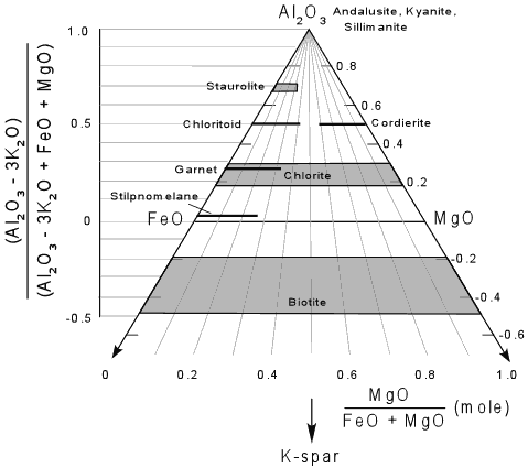
To calculate the plotting parameters for the AFM diagram the following
formulae are used:
Using these parameters, one can grid off the AFM diagram with the vertical scale represented by the normalized values for the A parameter -
and the horizontal position based on the ratio of MgO/(FeO + Mg). as seem below. Of course these values are obtained after converting the chemical analysis of the rock to molecular proportions. |
 |
| Note that if we project K-spar from muscovite, that the arrow points toward the K corner of the 4 component tetrahedron, and thus K-spar would project away from the front face of the diagram. Thus, as seen on the AFM face, K-spar would plot at negative infinity. |
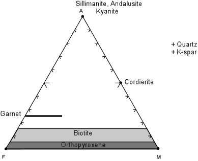
| The projection from muscovite works well for metamorphic rocks that contain muscovite. But, at higher grades of metamorphism, in the upper amphibolite facies and the granulite facies, muscovite becomes unstable and is replaced by K-feldspar + quartz + an Al2SiO5 mineral. In order to show rocks and mineral assemblages at these higher grades of metamorphism, a new projection is made from K-spar, as shown below. |
For this diagram the plotting parameters are much more straight forward,
with -
All on a molecular basis and then renormalized to sum to 100%. Note the absence of all hydrous phases (staurolite, chloritoid, muscovite) except biotite in this projection. |
 |
|
Resolving Problems As soon as we start ignoring components or projecting into three component composition diagrams there is a potential to lose information. Sometimes the loss of information creates a dilemma that must be resolved in order to understand the mineral assemblage. For example, a common medium grade assemblage in a pelitic rock is staurolite, garnet, muscovite, biotite, quartz, and plagioclase. Plotting these minerals on ACF, AKF, and AMF diagrams, as shown below creates a problem. For divariant equilibrium we expect the number of components to equal the number of phases (c=3, so p=3) at least for the ternary part of our system. Thus, in the ACF diagram, a rock like composition x would have plagioclase, garnet, staurolite (+quartz + muscovite), but biotite cannot be resolved from garnet because they plot near the same point(s). Still, in the ACF diagram, x plots within a 3 phase triangle. |
 |
|
In the AFM diagram the same rock of composition x is seen to have garnet, staurolite, and biotite (+quartz + muscovite). Plagioclase is ignored by the diagram (because CaO is not plotted), but we can resolve biotite and garnet because they clearly have different compositions in the AFM plot. In the AKF plot there is an ambiguity. Composition x plots in the correct 4 phase field of muscovite, garnet, staurolite, and Biotite, but divariant equilibrium requires that it plot in a 3 phase triangle. The problem in the AKF diagram implies one of the following:
Because the mineral assemblage is very common in medium grade pelitic rocks, it is unlikely that equilibrium has not been achieved, and it is unlikely that it represents a univariant assemblage (univariant assemblages are rare compared to divariant assemblages. |
|
Note that the AFM plot does show the proper assemblage, which suggests that the Fe and Mg components behave as separate components. In calculating the AKF and ACF diagrams we have combined Fe and Mg. Thus, neither the AKF nor the ACF diagrams truly represent a three component system, and this results in the ambiguity. While all of these diagrams are useful, we must always remember that the diagrams are simplifications of a more complex system, and thus, when ambiguities appear, one must apply reason to figure out why the diagrams do not explain what is observed in the rock. |
|
Examples of questions on this material that could be asked on an exam
|